Mumford on Math

"Mathematicians believe in this Platonic universe in that, there is a pre-existing bunch of facts which are true and you never invent anything, you are discovering".

Optical Flow, Lucas Kanade in Python

Following is the Lucas Kanade optical flow algorithm in Python. We used it successfully on two png images, as well as through OpenCV to follow a point in successive frames. More details are at Github.

import numpy as np
import scipy.signal as si
from PIL import Image

def gauss_kern():
   h1 = 15
   h2 = 15
   x, y = np.mgrid[0:h2, 0:h1]
   x = x-h2/2
   y = y-h1/2
   sigma = 1.5
   g = np.exp( -( x**2 + y**2 ) / (2*sigma**2) );
   return g / g.sum()

def deriv(im1, im2):
   g = gauss_kern()
   Img_smooth = si.convolve(im1,g,mode='same')
   fx,fy=np.gradient(Img_smooth)  
   ft = si.convolve2d(im1, 0.25 * np.ones((2,2))) + \
       si.convolve2d(im2, -0.25 * np.ones((2,2)))
                 
   fx = fx[0:fx.shape[0]-1, 0:fx.shape[1]-1]  
   fy = fy[0:fy.shape[0]-1, 0:fy.shape[1]-1];
   ft = ft[0:ft.shape[0]-1, 0:ft.shape[1]-1];
   return fx, fy, ft

import matplotlib.pyplot as plt
import numpy as np
import scipy.signal as si
from PIL import Image
import deriv
import numpy.linalg as lin

def lk(im1, im2, i, j, window_size) :
   fx, fy, ft = deriv.deriv(im1, im2)
   halfWindow = np.floor(window_size/2)
   curFx = fx[i-halfWindow-1:i+halfWindow,
              j-halfWindow-1:j+halfWindow]
   curFy = fy[i-halfWindow-1:i+halfWindow,
              j-halfWindow-1:j+halfWindow]
   curFt = ft[i-halfWindow-1:i+halfWindow,
              j-halfWindow-1:j+halfWindow]
   curFx = curFx.T
   curFy = curFy.T
   curFt = curFt.T

   curFx = curFx.flatten(order='F')
   curFy = curFy.flatten(order='F')
   curFt = -curFt.flatten(order='F')
 
   A = np.vstack((curFx, curFy)).T
   U = np.dot(np.dot(lin.pinv(np.dot(A.T,A)),A.T),curFt)
   return U[0], U[1]

Plotting a Complex Exponential

We rewrote one of the MIT OCW 18.03 ODE Mathlets in Python. This mathlet was for plotting complex exponentials.

from pylab import *

from matplotlib.widgets import Slider



ax = subplot(121)

subplots_adjust(left=0.1, bottom=0.25)

l1, = plot(None,None, lw=2, color='red')

axis([-1, 1, -8, 8])

title ('$(a + bi)t$', color='blue')

grid()



ax = subplot(122)

subplots_adjust(left=0.1, bottom=0.25)

l2, = plot(None,None, lw=2, color='red')

axis([-3, 3, -3, 3])

title ('$e^{(a + bi)t}$', color='blue')

grid()



axcolor = 'lightgoldenrodyellow'

axa = axes([0.15, 0.1, 0.65, 0.03], axisbg=axcolor)

axb  = axes([0.15, 0.15, 0.65, 0.03], axisbg=axcolor)



slidera = Slider(axa, 'a', -1.0, 1.0, valinit=0)

sliderb = Slider(axb, 'b', -8.0, 8.0, valinit=0)



def update(val):

    a = slidera.val

    b = sliderb.val

    t = arange(-1.0, 1.0, 0.001)

    l1.set_xdata(t)

    l1.set_ydata((b/a)*t)



    t = arange(-3.0, 3.0, 0.001)

    l2.set_xdata(exp(a*t)*cos(b*t))

    l2.set_ydata(exp(a*t)*sin(b*t))

    draw()



slidera.on_changed(update)

sliderb.on_changed(update)



show()

Clustering, Image Segmentation, Eigenvectors and Python

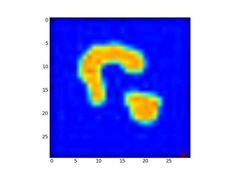
Here is example code for eigenvector based segmentation in Python. For more details, see code here.

import matplotlib.pyplot as plt
import numpy as np

Img = plt.imread("twoObj.jpg")
n = Img.shape[0]
Img2 = Img.flatten(order='C')
nn = Img2.shape[0]

A = np.zeros((nn,nn))

for i in range(nn):
 for j in range(nn):
     A[i,j]=np.exp(-((Img2[i]-Img2[j])**2))

V,D = np.linalg.eig(A)
V = np.real(V)
a = np.real(D[0])
print a

threshold = 0 # filter
a = np.reshape(a, (n,n))
Img[a<threshold] = 255
plt.imshow(Img)
plt.show()